Tablor.sty est un paquet conçu par Guillaume CONNAN pour générer automatiquement le tableau de signes ou le tableau de variations d’une fonction donnée.
Le paquet pro-tablor n’est qu’une adaptation pour être utiliser dans professor.sty.
Dans le préambule
On rajoute ceci :
\usepackage[xcas]{pro-tablor}
LES TABLEAUX DE VARIATIONS
TV
Fonction simple :
\begin{TV}
TV([-5,7],[],"f","x",x^2,0,n,\tv);
\end{TV}
On obtient :

TV
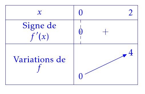
En couleur :
\coultab{blue}
\begin{TV}
TV([0,2],[],"f","x",x^2,1,n,\tv);
\end{TV}
On obtient :
TV
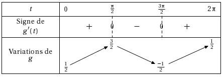
Fonction trigo :
\begin{TV}
   TV([0,2*pi],[],"g","t",sin(2*x)+x/2,1,t,\tv)
 \end{TV}
On obtient :
TVS
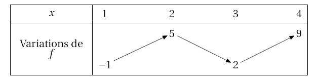
Tableau de variation à partir d’une liste d’abscisses et d’une liste d’images :
\begin{TVS}
TVS([1,2,3,4],[-1,5,2,9],[],"f","x",\tv)
\end{TVS}
On obtient :
ou encore :
\begin{TVS}
TVS([1,2,3,4],[-1,-infinity,+infinity,2,9],[2],"f","x",\tv)
\end{TVS}
On obtient :

TVPC
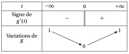
Fonction prolongeable par continuité. (Nouveauté 20/10/2008)
Par exemple pour $x\mapsto e^-1/x^2$, on entre trois listes :
– l’intervalle d’étude ;
– les valeurs où la fonction est prolongeable par continuité ;
– les valeurs où la dérivée n’est pas définie.
Le reste est comme dans TV.
\begin{TVPC}
TVPC([-infinity,+infinity],[0],[0],"g","t",e^(-1/x^2),1,n,\tv);
\end{TVPC}
On obtient :
TVZ
Fonction avec une zone interdite :
\begin{TVZ}
  TVZ([-infinity,+infinity],[],[[-1,1]],"f","x",sqrt(x^2-1),1,n,\tv)
\end{TVZ}
On obtient :

TVI
Tableau de fonction avec le théorème des valeurs intermédiaires :
\begin{TVI}
TVI([-10,+infinity],[-1,1],"f","x",x^2/(x^2-1),1,10,n,\tv)
\end{TVI}
On obtient :
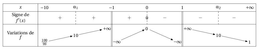
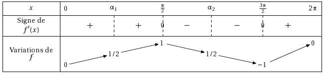
Tableau de fonction trigo avec le théorème des valeurs intermédiaires :
\begin{TVI}
   TVI([0,2*pi],[],"f","x",sin(x),1,1/2,t,\tv)
 \end{TVI}
On obtient :
TVIex
Tableau de fonction avec le théorème des valeurs intermédiaires avec racines exactes:
\begin{TVIex}
  TVIex([0,2*pi],[],"f","x",sin(x),1,1/2,t,\tv)
\end{TVIex}
On obtient :
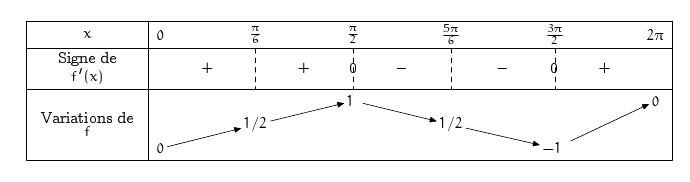
Tableau de variations avec valeurs approchées.
\begin{TVapp}
TVapp([0,+infinity],[0],"g","x",ln(x)-x*exp(2-x),1,n,\tv)
\end{TVapp}
On obtient :

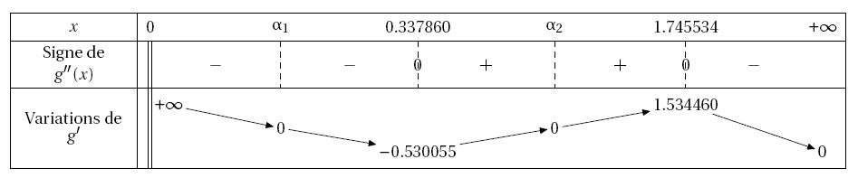
TVIapp
\begin{TVIapp}
 TVIapp([0,+infinity],[0],"g'","x",diff(ln(x)-x*exp(2-x),x),1,n,\tv)
\end{TVIapp}
On obtient :
LES COURBES PARAMÉTRÉES
TVP (premier exemple)
Fonction paramétrée :
\begin{TVP}
 TVP([0,pi/2],[[],[]],["x","y"],"t",[cos(3*t),sin(4*t)],1,t,\tv)
 \end{TVP}
On obtient :

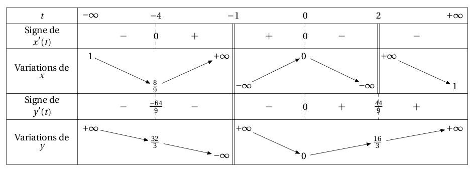
TVP (deuxième exemple)
Fonction paramétrée :
\begin{TVP}
TVP([-infinity,+infinity],[[-1,2],[-1]],["x","y"],"t",[t^2/((t+1)*(t-2)),t^2*(t+2)/(t+1)],1,0,\tv)
\end{TVP}
On obtient :
LES TABLEAUX DE SIGNES
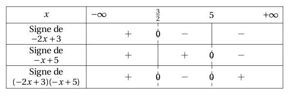
TSa
Cas du produit de deux facteurs affines :
\begin{TSa}
TSa(-2,3,-1,5,\tv);
\end{TSa}
On obtient :
TS
Autres produits :
\begin{TS}
TS("P",[-2*x+3,x^2-1,x^2+1,x-1,x^2-2],[-infinity,+infinity],n,\tv);
\end{TS}
On obtient :

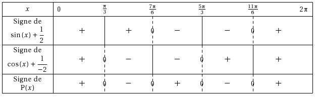
Avec des fonctions trigo :
\begin{TS}
TS("P",[sin(x)+1/2,cos(x)-1/2],[0,2*pi],t,\tv)
\end{TS}
On obtient :
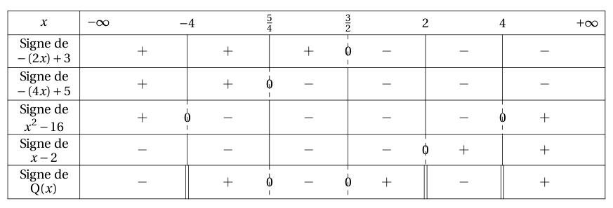
TSq
Quotient :
\begin{TSq}
TSq("Q",[-2*x+3,-4*x+5],[x^2-16,x-2],[-infinity,+infinity],n,\tv)
\end{TSq}
On obtient :
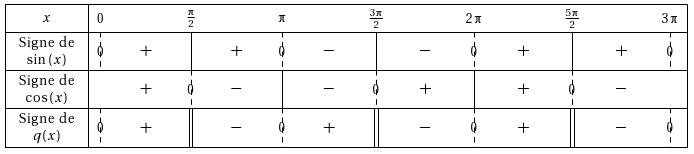
Quotient trigo :
\begin{TSq}
   TSq("q",[sin(x)],[cos(x)],[0,3*pi],t,\tv)
\end{TSq}
On obtient :
TSc
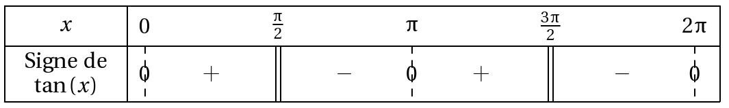
Pour un tableau de signe à une seule ligne :
\begin{TSc}
TSc(tan(x),[0,2*pi],[pi/2,3*pi/2],t,\tv)
\end{TSc}
On obtient :
Réduction d’échelle
Pour réduire la taille d’un tableau, on utilise la commande \ech sans oublier de remettre à l’échelle 1 ensuite :
\ech{0.8}
\begin{TS}
TS("P",[sin(x)+1/2,cos(x)-1/2,cos(x)-sqrt(3)/2],[0,3*pi/2],t,\tv)
\end{TS}
\ech{1}
On obtient :